Pass Or Fail Problem¶

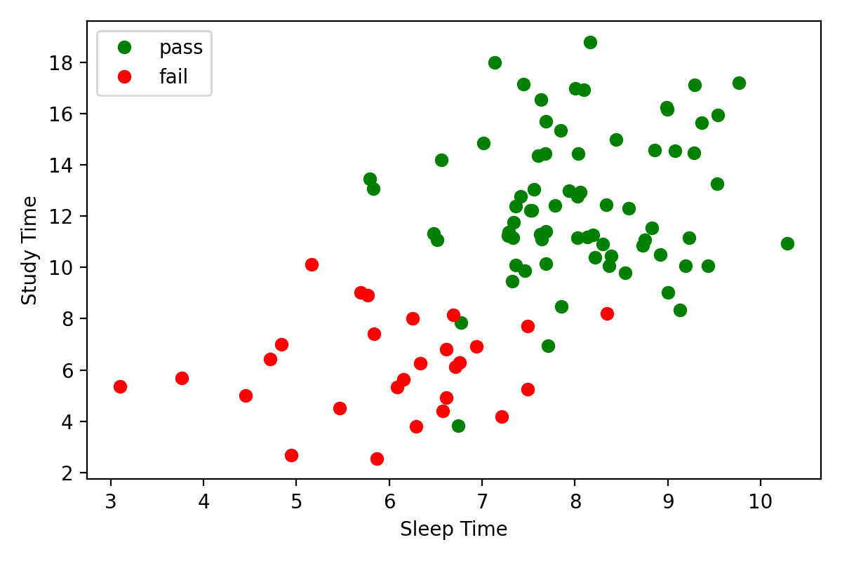
A class of 100 students takes an exam. At the end of the exam, the students self-report the number of hours they studied for the exam and the amount of sleep they got the night before. Here's what the data looks like including the Pass/Fail exam results.

import numpy as np

# random number generator
rng = np.random.default_rng(123)

# data (72 passes / 28 fails)
passes_sleep = rng.normal(loc=8, scale=1, size=72)
passes_study = rng.normal(loc=12, scale=3, size=72)
fails_sleep = rng.normal(loc=6, scale=1.5, size=28)
fails_study = rng.normal(loc=6, scale=2, size=28)

Pass vs Fail Plot

import matplotlib.pyplot as plt

fig, ax = plt.subplots()
ax.plot(passes_sleep, passes_study, linestyle='None', marker='o', color='g', label='pass')
ax.plot(fails_sleep, fails_study, linestyle='None', marker='o', color='r', label='fail')
ax.set_xlabel('Sleep Time')
ax.set_ylabel('Study Time')
ax.legend()

Design and fit a logistic regression model to this data. Be sure to subclass nn.Module.

Here's some starter code.

import torch
from torch import nn

# set random seed for reproducibility
torch.manual_seed(0)

class LogisticRegression(nn.Module):
    """
    Logistic Regression model of the form 1/(1 + e^-(w1x1 + w2x2 + ...wnxn + b))
    """

    pass

Perceptron vs Logistic Regression

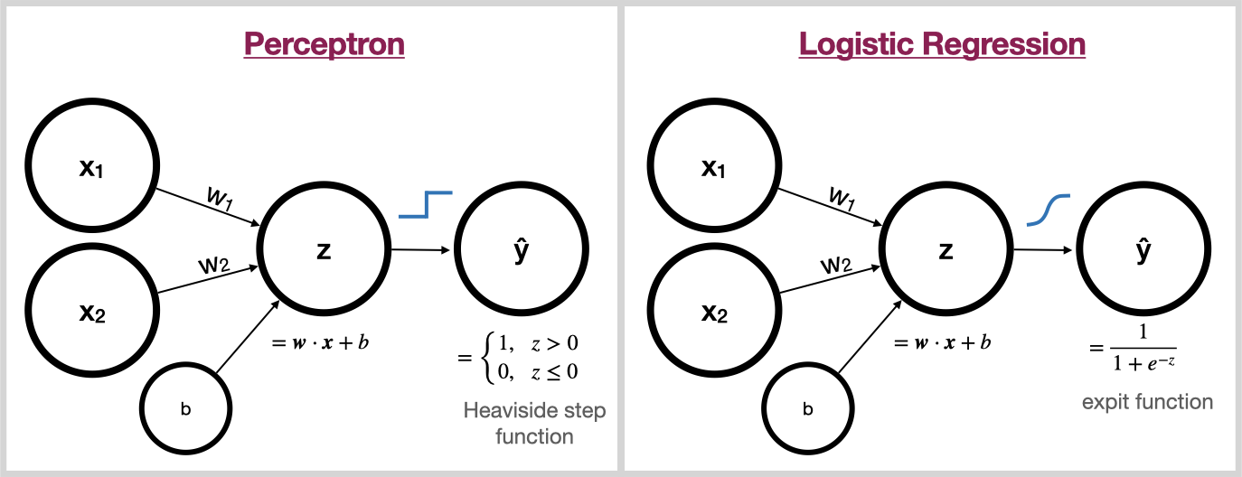
Notice the striking similarity between the Perceptron and Logistic Regression. The only difference is, the Perceptron uses the Heaviside step function to squash its input into the discrete set {0, 1} whereas Logistic Regression uses the expit function to squash its input into the continuous range (0,1).

This effect of this is, Logistic Regression is differentiable and the Perceptron is not! Therefore, logistic regression can be trained with gradient descent while the Perceptron relies on other learning algorithms.

Bonus 1¶

Use your fitted model to make predictions on the following test data.

test_sleep = np.array([
    7.06, 7.19, 7.59, 8.84, 9.66, 9.72, 8.81,
    8.44, 5.66, 9.13, 8.04, 5.31, 7.07, 8.33, 7.83
])
test_study = np.array([
    19.89, 13.36, 12.7, 14.1, 14.19, 12.4, 10.88, 
    13.09, 7.88, 6.35, 4.89, 6.65, 3.67, 5.79, 8.09
])

Bonus 2¶

Draw your fitted model's decision boundary onto the plot above.

Try with Google Colab